Linear Regression Models
- 1. Introduction
- 2. The Simple Linear Regression Model
- 3. Method of Least Squares
- 4. Derivation of \(\hat{\beta}_0\) and \(\hat{\beta}_1\)
- 5. Quality of the Regression
- 6. Properties of Least-Squares Estimators
- 7. Estimation of Error Variance \(\sigma^2\)
- 8. Inference on Least Squares Estimators
- 9. ANOVA Approach to Regression
- 10. Predicting a Particular Value of \(Y\)
- 11. Correlation Analysis
- 12. Matrix Notation for Linear Regression
- 13. ANOVA for Multiple Regression
- 14. Regression Diagnostics
- 15. Applications
- 16. Conclusion
1. Introduction
Few statistical techniques have shaped data analysis and machine learning as profoundly as linear regression. Though it can appear deceptively simple—fitting a line (or hyperplane) to data points—linear regression underpins some of the most important ideas in supervised learning, inference, and statistical modeling. From the earliest developments by Carl Friedrich Gauss and Adrien-Marie Legendre in the early 19th century (when they applied the method of least squares to astronomical observations), linear regression has matured into a rigorous framework that touches on everything from basic correlation to multivariate interpretability.
In this comprehensive guide, we’ll explore the key building blocks:
- Simple Linear Regression: Understanding the relationship between a single predictor and a response variable.
- Method of Least Squares: Deriving how the best-fitting line (or hyperplane) is found by minimizing the sum of squared residuals.
- Inference: Determining confidence intervals, conducting hypothesis tests (e.g., is a slope significantly different from zero?), and analyzing variance components via ANOVA.
- Properties: Learning why least-squares estimators are unbiased, consistent, and how we estimate unknown parameters like \(\sigma^2\).
- Matrix Notation: Scaling up from a single predictor to many, with the regression model expressed in matrix form.
- Diagnostics & Applications: Checking model assumptions, dealing with outliers, exploring real-world use cases in machine learning (feature selection, interpretability, etc.).
We’ll also keep the mathematical rigor at the forefront, ensuring that each formula is clearly stated with double-dollar notation for clarity. By the end, you’ll see how linear regression remains a cornerstone of data science and an intuitive gateway to more advanced modeling techniques.
2. The Simple Linear Regression Model
2.1 Setup and Notation
In its most basic form, simple linear regression models the relationship between:
- A single predictor (independent variable) \(x\).
- A response (dependent variable) \(y\).
We assume a linear relationship of the form:
\[y_i = \beta_0 + \beta_1 x_i + \varepsilon_i, \quad i = 1, 2, \ldots, n.\]Here:
- \(\beta_0\) is the intercept (the value of \(y\) when \(x = 0\)).
- \(\beta_1\) is the slope (the rate of change in \(y\) per unit of \(x\)).
- \(\varepsilon_i\) are the errors or residuals, which we typically assume to be i.i.d. normal with mean 0 and variance \(\sigma^2\).
Hence, the model can be stated as:
\[y_i = \beta_0 + \beta_1 x_i + \varepsilon_i, \quad \varepsilon_i \sim \mathcal{N}(0, \sigma^2).\]2.2 Visual Representation
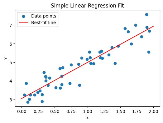
Imagine plotting data points \((x_i, y_i)\) on a scatterplot. A simple linear regression tries to place a straight line that best fits these points in a least-squares sense.
- Line: \(\hat{y} = \hat{\beta}_0 + \hat{\beta}_1 x\)
- Residual: The vertical distance from a data point to the fitted line: \(e_i = y_i - \hat{y}_i\).
Below, we’ll generate a small synthetic dataset, fit a simple linear regression in Python, and then create a scatter plot overlaid with the best-fit line. We assume you have numpy and matplotlib installed.
import numpy as np
import matplotlib.pyplot as plt

# 1. Generate synthetic data
np.random.seed(42)
n = 50
x = 2 * np.random.rand(n, 1)  # predictor
# True relationship: y = 3 + 2*x + some noise
y = 3 + 2 * x + np.random.randn(n, 1) * 0.5

# 2. Fit a simple linear regression via the normal equations
# X design matrix: first column of 1s for intercept, plus x
X = np.c_[np.ones((n, 1)), x]  # shape (50, 2)
# Solve for beta using (X^T X)^{-1} X^T y
beta_hat = np.linalg.inv(X.T.dot(X)).dot(X.T).dot(y)

# Extract fitted intercept and slope
beta0_hat = beta_hat[0, 0]
beta1_hat = beta_hat[1, 0]

print("Estimated intercept:", beta0_hat)
print("Estimated slope:", beta1_hat)

# 3. Plot data and regression line
plt.figure(figsize=(6, 4))
plt.scatter(x, y, label="Data points")
# For the regression line, create a sequence of x-values, then predict y
x_new = np.linspace(0, 2, 100).reshape(-1, 1)
X_new = np.c_[np.ones((100, 1)), x_new]
y_pred = X_new.dot(beta_hat)

plt.plot(x_new, y_pred, color="red", label="Best-fit line")
plt.xlabel("x")
plt.ylabel("y")
plt.title("Simple Linear Regression Fit")
plt.legend()
plt.show()

- Explanation:
- Data Generation: We create 50 points from the true model \(y = 3 + 2x + \varepsilon\), with some Gaussian noise.
- Fitting: We set up the design matrix \(\mathbf{X}\) (with a column of 1s for the intercept) and solve for
\(\hat{\boldsymbol{\beta}} = (\mathbf{X}^\top \mathbf{X})^{-1}\mathbf{X}^\top \mathbf{y}.\) - Visualization: We scatter-plot the data and overlay the regression line in red.
3. Method of Least Squares
The method of least squares chooses \(\hat{\beta}_0, \hat{\beta}_1\) so as to minimize the sum of squared residuals. Specifically, define:
\[S(\beta_0, \beta_1) = \sum_{i=1}^n \bigl(y_i - (\beta_0 + \beta_1 x_i)\bigr)^2.\]We want:
\[(\hat{\beta}_0, \hat{\beta}_1) = \arg \min_{\beta_0, \beta_1} \; S(\beta_0, \beta_1).\]In more intuitive terms, least squares penalizes large deviations heavily by squaring them. Thus, we find the line that keeps these squared deviations as small as possible across all data points.
4. Derivation of \(\hat{\beta}_0\) and \(\hat{\beta}_1\)
4.1 Minimizing the Sum of Squared Errors
Start with:
\[S(\beta_0, \beta_1) = \sum_{i=1}^n \bigl(y_i - \beta_0 - \beta_1 x_i\bigr)^2.\]To find the minimum, we set partial derivatives to zero:
\[\frac{\partial S}{\partial \beta_0} = 0, \quad \frac{\partial S}{\partial \beta_1} = 0.\]Partial derivative wrt \(\beta_0\)
\[\frac{\partial}{\partial \beta_0} \sum_{i=1}^n (y_i - \beta_0 - \beta_1 x_i)^2 = -2 \sum_{i=1}^n (y_i - \beta_0 - \beta_1 x_i).\]Set it to 0:
\[\sum_{i=1}^n (y_i - \beta_0 - \beta_1 x_i) = 0 \quad \Longrightarrow \quad \sum_{i=1}^n y_i - n\beta_0 - \beta_1 \sum_{i=1}^n x_i = 0.\]So:
\[n \hat{\beta}_0 + \hat{\beta}_1 \sum_{i=1}^n x_i = \sum_{i=1}^n y_i. \quad (1)\]Partial derivative wrt \(\beta_1\)
\[\frac{\partial}{\partial \beta_1} \sum_{i=1}^n (y_i - \beta_0 - \beta_1 x_i)^2 = -2 \sum_{i=1}^n x_i (y_i - \beta_0 - \beta_1 x_i).\]Set it to 0:
\[\sum_{i=1}^n x_i (y_i - \beta_0 - \beta_1 x_i) = 0 \quad \Longrightarrow \quad \sum_{i=1}^n x_i y_i - \beta_0 \sum_{i=1}^n x_i - \beta_1 \sum_{i=1}^n x_i^2 = 0.\]So:
\[\hat{\beta}_0 \sum_{i=1}^n x_i + \hat{\beta}_1 \sum_{i=1}^n x_i^2 = \sum_{i=1}^n x_i y_i. \quad (2)\]4.2 Solving the Normal Equations
Equations (1) and (2) are called the normal equations. We can solve them simultaneously. Let:
\[\bar{x} = \frac{1}{n} \sum_{i=1}^n x_i, \quad \bar{y} = \frac{1}{n} \sum_{i=1}^n y_i.\]Then, we can show:
\[\hat{\beta}_1 = \frac{\sum_{i=1}^n (x_i - \bar{x})(y_i - \bar{y})}{\sum_{i=1}^n (x_i - \bar{x})^2} = \frac{ \sum_{i=1}^n x_i y_i - n \bar{x}\,\bar{y} } { \sum_{i=1}^n x_i^2 - n \bar{x}^2 }.\]and
\[\hat{\beta}_0 = \bar{y} - \hat{\beta}_1 \bar{x}.\]Thus:
- Slope: \(\hat{\beta}_1\) is the ratio of the covariance between \(x\) and \(y\) to the variance of \(x\).
- Intercept: \(\hat{\beta}_0\) ensures that the fitted line passes through the point \((\bar{x}, \bar{y})\).
5. Quality of the Regression
5.1 Residuals and \(R^2\)
Once we fit the line \(\hat{y}_i = \hat{\beta}_0 + \hat{\beta}_1 x_i\), we can examine:
- Residual: \(e_i = y_i - \hat{y}_i.\)
- Sum of Squared Residuals: \(\text{SSR} = \sum_{i=1}^n e_i^2.\)
- Total Sum of Squares: \(\text{SST} = \sum_{i=1}^n (y_i - \bar{y})^2.\)
- Regression Sum of Squares: \(\text{SSRg} = \sum_{i=1}^n (\hat{y}_i - \bar{y})^2.\)
The well-known identity is:
\[\text{SST} = \text{SSRg} + \text{SSR}.\]We often measure the “proportion of variance explained” by:
\[R^2 = \frac{\text{SSRg}}{\text{SST}} = 1 - \frac{\text{SSR}}{\text{SST}}.\]- \(R^2\) closer to 1 indicates that the model explains a high fraction of the variability in \(y\).
- \(R^2\) near 0 means the model explains little of that variability.
5.2 Residual Plots
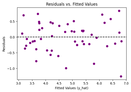
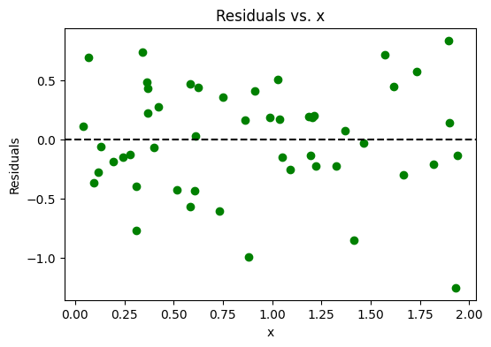
Residual plots help check whether the residuals exhibit any pattern (suggesting nonlinearity or heteroscedasticity) and whether they appear randomly scattered. Here’s a snippet to create residual vs. predicted and residual vs. x plots.
# Assuming you've already fit beta_hat as above
# 1. Compute residuals
y_hat = X.dot(beta_hat)        # fitted values
residuals = y - y_hat          # vector of residuals

# 2. Plot residuals vs. fitted values
plt.figure(figsize=(6, 4))
plt.scatter(y_hat, residuals, color="purple")
plt.axhline(y=0, color="black", linestyle="--")
plt.xlabel("Fitted Values (y_hat)")
plt.ylabel("Residuals")
plt.title("Residuals vs. Fitted Values")
plt.show()

# 3. Plot residuals vs. x
plt.figure(figsize=(6, 4))
plt.scatter(x, residuals, color="green")
plt.axhline(y=0, color="black", linestyle="--")
plt.xlabel("x")
plt.ylabel("Residuals")
plt.title("Residuals vs. x")
plt.show()


- Interpretation:
- A horizontal band of points around zero, with no distinct pattern, suggests the model’s linearity and constant variance assumptions may hold.
- If you see a clear curve or fanning shape, it might indicate a violation (e.g., nonlinearity or changing variance).
6. Properties of Least-Squares Estimators
Under the classical linear model assumptions:
- Linearity: \(y_i = \beta_0 + \beta_1 x_i + \varepsilon_i.\)
- Independent errors: \(\varepsilon_i\) are independent.
- Zero mean: \(E[\varepsilon_i] = 0.\)
- Constant variance: \(\mathrm{Var}(\varepsilon_i) = \sigma^2.\)
- No exact multicollinearity (in the multiple regression sense).
Then:
-
Unbiasedness:
\(E[\hat{\beta}_1] = \beta_1, \quad E[\hat{\beta}_0] = \beta_0.\) -
Variance:
\(\mathrm{Var}(\hat{\beta}_1) = \frac{\sigma^2}{\sum_{i=1}^n (x_i - \bar{x})^2}, \quad \mathrm{Var}(\hat{\beta}_0) = \sigma^2 \biggl[\frac{1}{n} + \frac{\bar{x}^2}{\sum (x_i - \bar{x})^2}\biggr].\) -
Best Linear Unbiased Estimator (BLUE): By the Gauss-Markov theorem, the ordinary least squares (OLS) estimators \(\hat{\beta}_0, \hat{\beta}_1\) have the smallest variance among all linear unbiased estimators.
7. Estimation of Error Variance \(\sigma^2\)
We don’t typically know \(\sigma^2\) beforehand. A natural estimator is the residual mean squared error:
\[\hat{\sigma}^2 = \frac{1}{n - 2} \sum_{i=1}^n (y_i - \hat{y}_i)^2 = \frac{\text{SSR}}{n - 2}.\]We divide by \((n-2)\) (instead of \(n\)) because we have estimated 2 parameters (\(\beta_0, \beta_1\)) from the data. This ensures unbiasedness under the classical assumptions:
\[E[\hat{\sigma}^2] = \sigma^2.\]8. Inference on Least Squares Estimators
8.1 Confidence Intervals for \(\beta_1\)
Under the assumption that \(\varepsilon_i\) are i.i.d. normal,
\[\frac{\hat{\beta}_1 - \beta_1}{\sqrt{\mathrm{Var}(\hat{\beta}_1)}} \sim t_{n-2}.\]Hence, a (1 – \(\alpha\)) confidence interval for \(\beta_1\) is:
\[\hat{\beta}_1 \pm t_{\alpha/2,\,n-2} \sqrt{\mathrm{Var}(\hat{\beta}_1)},\]where \(t_{\alpha/2,\,n-2}\) is the critical value from the Student’s t distribution with \((n-2)\) degrees of freedom.
8.2 Hypothesis Test for \(\beta_1\)
- Null: \(H_0: \beta_1 = 0\) (no linear relationship between \(x\) and \(y\)).
- Alternative: \(H_a: \beta_1 \neq 0\) (two-sided) or \(\beta_1 > 0\) or \(\beta_1 < 0\) (one-sided).
We compute:
\[T = \frac{\hat{\beta}_1 - 0}{\sqrt{\mathrm{Var}(\hat{\beta}_1)}},\]| and compare with a t distribution with \((n-2)\) degrees of freedom. If $$ | T | \(is large, we reject\)H_0\(and conclude\)\beta_1$$ is significantly different from zero. |
8.3 Confidence Interval for \(\beta_0\)
A similar procedure applies for \(\beta_0\). We use:
\[\mathrm{Var}(\hat{\beta}_0) = \hat{\sigma}^2 \Bigl[\frac{1}{n} + \frac{\bar{x}^2}{\sum_{i=1}^n (x_i - \bar{x})^2}\Bigr],\]and again we rely on a \(t_{n-2}\) distribution for inference.
9. ANOVA Approach to Regression
9.1 Analysis of Variance Decomposition
We can treat the linear regression in an ANOVA framework:
- Total Variation in \(y\): \(\text{SST} = \sum (y_i - \bar{y})^2.\)
- Explained Variation: \(\text{SSRg} = \sum (\hat{y}_i - \bar{y})^2.\)
- Unexplained Variation: \(\text{SSR} = \sum (y_i - \hat{y}_i)^2.\)
Hence:
\[\text{SST} = \text{SSRg} + \text{SSR}.\]9.2 F-Test for Regression
We can test overall regression significance:
\[F = \frac{\text{SSRg}/1}{\text{SSR}/(n-2)} = \frac{\text{SSRg}}{\text{SSR}} \times (n-2).\]Under \(H_0: \beta_1 = 0\), the statistic follows an \(F_{1,\,n-2}\) distribution. If \(F\) is large, we reject \(H_0\). This is equivalent to the two-sided t-test for \(\beta_1\) but in an ANOVA format.
10. Predicting a Particular Value of \(Y\)
Often we want to predict \(y_{\text{new}}\) at a specific \(x = x_{\text{new}}\). The fitted model gives:
\[\hat{y}_{\text{new}} = \hat{\beta}_0 + \hat{\beta}_1 x_{\text{new}}.\]10.1 Prediction Interval vs. Confidence Interval
-
Confidence interval for the mean response at \(x_{\text{new}}\):
\[\hat{y}_{\text{mean,new}} \pm t_{\alpha/2,\,n-2} \; \sqrt{\mathrm{Var}(\hat{y}_{\text{mean,new}})},\]where
\[\mathrm{Var}(\hat{y}_{\text{mean,new}}) = \hat{\sigma}^2 \Bigl[ \frac{1}{n} + \frac{(x_{\text{new}} - \bar{x})^2}{\sum (x_i - \bar{x})^2} \Bigr].\] -
Prediction interval for an individual new observation is wider because it includes the irreducible error \(\sigma^2\). So:
\[\hat{y}_{\text{new}} \pm t_{\alpha/2,\,n-2} \; \sqrt{ \hat{\sigma}^2 \Bigl[ 1 + \frac{1}{n} + \frac{(x_{\text{new}} - \bar{x})^2}{\sum (x_i - \bar{x})^2} \Bigr] }.\]
11. Correlation Analysis
In simple linear regression, the correlation coefficient between \(x\) and \(y\) is:
\[r = \frac{\sum_{i=1}^n (x_i - \bar{x})(y_i - \bar{y})} {\sqrt{\sum (x_i - \bar{x})^2 \; \sum (y_i - \bar{y})^2}}.\]We have an important relationship:
\[r = \pm \sqrt{R^2},\]where the sign depends on the slope’s sign (\(\hat{\beta}_1\)).
- If \(r\) is close to +1 or -1, we have a strong linear relationship.
- If \(r\) is near 0, it suggests little linear correlation (though not necessarily independence).
12. Matrix Notation for Linear Regression
When we move from simple regression to multiple regression with \(k\) predictors, we typically write:
\[\mathbf{y} = \mathbf{X}\boldsymbol{\beta} + \boldsymbol{\varepsilon},\]where:
- \(\mathbf{y}\) is an \(n \times 1\) vector of responses.
- \(\mathbf{X}\) is an \(n \times (k+1)\) design matrix (the first column is all 1s for the intercept, plus columns for each predictor).
- \(\boldsymbol{\beta}\) is a \((k+1) \times 1\) vector of unknown parameters:
\(\boldsymbol{\beta} = \begin{bmatrix} \beta_0 \\ \beta_1 \\ \vdots \\ \beta_k \end{bmatrix}.\) - \(\boldsymbol{\varepsilon}\) is an \(n \times 1\) vector of error terms.
12.1 Least Squares Solution
The method of least squares in matrix form solves:
\[\min_{\boldsymbol{\beta}} \; (\mathbf{y} - \mathbf{X}\boldsymbol{\beta})^\top (\mathbf{y} - \mathbf{X}\boldsymbol{\beta}).\]Taking derivatives and setting to zero yields the normal equations:
\[\mathbf{X}^\top \mathbf{X} \;\hat{\boldsymbol{\beta}} = \mathbf{X}^\top \mathbf{y}.\]If \(\mathbf{X}^\top \mathbf{X}\) is invertible:
\[\hat{\boldsymbol{\beta}} = (\mathbf{X}^\top \mathbf{X})^{-1} \mathbf{X}^\top \mathbf{y}.\]12.2 Interpretations and Extensions
- We can still interpret \(\beta_j\) as the effect on \(y\) of a one-unit change in \(x_j\), holding other predictors constant.
- Covariances, confidence intervals, and F-tests generalize accordingly.
- The design matrix approach is the bedrock for advanced regression methods, including polynomial regression, interactions, or even linear models with transformations.
13. ANOVA for Multiple Regression
13.1 Decomposition
For multiple linear regression with \(k\) predictors:
- Total SS: \(\text{SST} = \sum_{i=1}^n (y_i - \bar{y})^2.\)
- Regression SS: \(\text{SSRg} = \sum_{i=1}^n (\hat{y}_i - \bar{y})^2.\)
- Error SS: \(\text{SSR} = \sum_{i=1}^n (y_i - \hat{y}_i)^2.\)
We still have:
\[\text{SST} = \text{SSRg} + \text{SSR}.\]13.2 F-Test
We can test the significance of all regression coefficients except the intercept:
\[F = \frac{\text{SSRg}/k}{\text{SSR}/(n-k-1)}.\]- If \(F\) is large, it implies at least one \(\beta_j \neq 0\) among \(j = 1, 2, \ldots, k\).
- Detailed partial F-tests can check subsets of predictors.
14. Regression Diagnostics
No real-world dataset perfectly meets all assumptions. Diagnostics ensure we check:
- Residual Plots: Are residuals randomly scattered? Or do we see patterns, indicating nonlinearity or heteroscedasticity?
- QQ-Plots: Do residuals appear normally distributed?
- Leverage and Influence: Are there data points with high leverage (extreme \(x\) values) or large influence on the fitted model? Tools like Cook’s distance help identify them.
- Multicollinearity: In multiple regression, highly correlated predictors can inflate standard errors. We measure this via variance inflation factors (VIFs).
If diagnostics suggest issues, we might transform variables, remove outliers carefully, or use robust regression techniques.
15. Applications
Having established the thorough mathematical foundation, let’s see how linear regression is deployed in modern machine learning and analytics workflows.
15.1 Regression Modeling in ML
Despite the prevalence of more complex models (random forests, neural networks), linear regression remains a mainstay:
- Baseline: Often the first step to benchmark a dataset’s predictability.
- Scalability: Huge datasets can be handled efficiently with linear solvers (like stochastic gradient descent).
- Online Learning: The linear model easily updates with streaming data if done via incremental learning approaches.
In ML, we might incorporate:
- Regularization: L2 (ridge), L1 (lasso), or elastic net to handle collinearity or feature selection.
- Polynomial Terms: Transform input features to capture nonlinearities while still solving a “linear in parameters” problem.
15.2 Feature Impact and Sensitivity
One of linear regression’s superpowers is interpretability:
- Coefficient \(\beta_j\) can be read as “the effect of feature \(x_j\) on the response, holding other features constant.”
- Standard errors and t-tests let us gauge each coefficient’s significance.
- Confidence intervals yield insight into the uncertainty around each effect estimate.
Data scientists often prefer linear models to black-box models precisely for this transparent look into why a prediction is made.
15.3 Multivariate Regression and Interpretability
When we extend from simple to multiple regression, we see:
- Interaction Terms: We might include \(x_1 x_2\) as an interaction term, capturing synergy between features.
- Dummy Variables / Encoding: For categorical predictors, we can incorporate them via dummy (0/1) variables.
- Multicollinearity: If two features are strongly correlated, their individual \(\beta_j\) estimates might be unstable. We then interpret them carefully or simplify the model (e.g., PCA prior to regression).
In real applications—like economic forecasting or medical analytics—the ability to interpret each coefficient helps domain experts trust the model’s conclusions.
16. Conclusion
Linear regression may appear straightforward—just finding the “best line” that connects points—but its reach extends far beyond the basics. By deriving and interpreting parameters like \(\hat{\beta}_0\) and \(\hat{\beta}_1\) , analyzing variance with ANOVA, and examining diagnostics, we gain both predictive power and insight into why certain patterns appear. That dual value—as both an inferential tool and a baseline predictive model—keeps linear regression front and center in modern analytics.
The term “regression” itself arose when Sir Francis Galton noticed that exceptionally tall parents tended to have somewhat shorter children, while exceptionally short parents often had somewhat taller children—both “regressing” toward more average heights. Although it began as an explanation of physical traits, the concept quickly expanded to describe how outcomes often drift back toward a mean. Today, the language of “regression” unifies everything from a one-predictor study of height vs. weight to high-dimensional industrial applications with countless features.
Ultimately, linear regression’s staying power lies in its balance of interpretability, mathematical clarity, and scalability. Whether serving as a first pass on new data or providing an interpretive lens for richer datasets, its simple premise—“model output as a linear combination of inputs plus error”—remains a bedrock concept. It reminds us that sometimes the oldest, most fundamental tools still yield the most enduring insights.